Topology - Continuity is a topological notion.

I was motivated by the discussion of topology and continuity found here:

http://scientopia.org/blogs/goodmath/2010/10/03/topological-spaces-and-continuity/

I would like to base on that discussion, and to bring my view of the subject:

I am not actually proving any thing, All I am trying to discuse is make the “if and only if” relation between the continuous function and respect of the open sets, more intuitive. I start from a point or intuitive claim that continious function is the function that maps near point to near points (\(f(\cdot)\) is continious if when \(t \rightarrow s\) (become nearer and nearer) then also \(f(t) \rightarrow f(s)\).

Once you are comfortable with the fact that topology defines nearness or neighborhoods you can think of continuous functions as functions that do not violate this neighborhoodness ( :) ). What I mean is that neighbors in the domain are also neighbors in codomain (image) (Of cause, there need to be topology in codomain). Think of it – the nearness is encoded using inclusions on open sets, Now the inclusion is never violated by functions, any function: if \(A \subset B\) and \(A,B \in\) doamin then \(f(A) \subset f(B) \in\) codomain.  So for the nearness to hold it is enough  to require that function \(f(\cdot)\) will respect open sets of domain – every open set in domain is also mapped to an open in codomain. In this scenario, you have no chose, but every encoded “nearness” in domain corresponds straight forward to the nearness in codomain, under change between elements of domain to elements of codomain done by \(f(\cdot)\).

So you may think of continuous function as translation that do not destroy neighbohoodness, indeed in case that the domain and codomain are same topological spaces, it is like deforming the space squeezing it like a rubber without tearing – also the rubber deforms the neighbors are never separated. Not destroing nearness just mean that – \(t \rightarrow s\) implies \(f(t) \rightarrow f(s)\)

“And do you, remember me?” ("А ты меня помнишь?") - poem by Andrei Voznesensky (Андрей Вознесенский)

 

Here you can find the translation - Chulpan Khamatova reading Andrei Voznesensky.

This is in such a contrast to all the classic poetry that it makes me wonder… Here nothing is said directly every thing is on the subconscious level. I don’t understand the “story” told in this poem yet, it does fell like some kind of retrospective on the long gone time, which does look happy (morning), naive and careless, from the today vintage point, the terrible midnight.

The last thing that always helps to go on in the dark routine is the knowledge, that there is a link which connect you to this past, and it is not mere a fruit of your imagination, this link is the other person that shared that time with you.

Ты мне прозвонилась сквозь страшную полночь: "А ты меня помнишь?" ну, как позабыть тебя, ангел-звереныш? "А ты меня помнишь?" твой голос настаивал, стонущ т тонущ - "А ты меня помнишь?" "А ты меня помнишь?" и ухало эхо во тьме телефонищ - рыдало по-русски, in English, in Polish- you promise? Astonish…а ты меня помнишь? А ты меня помнишь, дорога до Бронниц? И нос твой, напудренный утренним пончиком? В ночном самолете отстегнуты помочи - Вы, кресла, нас помните? Понять, обмануться, окликнуть по имени: А ты меня… Помнишь? Как скорая помощь, В беспамятном веке запомни одно лишь - "А ты меня помнишь?"

Don’t know when this poem was published.

Probability 7 - Fair gambling game

Seventh post in the series.

Fair gambling game

Fair gambling game is obviously a game that when you ask someone what his earnings will be before he starts to play he will tell you that it will be zero on average (otherwise the game system gives him some advantage over the “bank”, since if on average he is better off, this means that its not the luck that he may relay on but the gambling system prefers him over the “bank”)

Now this is tricky question, it will be crucial for the interpretation of rigorous mathematic approach to come - If you ask a gambler, a priori (you ask hin on time \(n=0\) before he even played his first bet), what will be, on average, his gain be on the \(n+1\) step (the surplus on this single bet) after he already have played \(n\) games? He will tell you it is still zero. And indeed, what difference it makes a priori to know that there will be moment in future where he has played \(n\) games? If it does make the difference Otherwise it is build into the system that before playing gambler already knows that after playing \(n\) games he on average wins in the next turn, making the whole game not fair.

In last post on probability I talked about filtration I tried to explain how filtration is related to information gathering as time progresses. I used the ability to answer questions regarding the outcome of events to illustrate the relation. Now the question previously asked can be stated as follows (combining the conditional expectation, that relay on appropriate filtration).

Suppose the gain per unit gamble on time \(n\) is given by random variable \(X_n\), Now our previous question rigorously translates to

• First question: \(\mathbb{E}[X_n]=0\)
• Second, the tricky one: \(\mathbb{E}[X_{n+1}|\mathcal{F_n}]=0 (a.s.)\)

Probability 6 - Predictable process

Sixth post in the series.

This post is natural sequel to the last post on relation of information and filtration.

Predictable Process

\(H_n\) is called a predictable process on filtration \(\{\mathcal{F}_n\}\) if for every \(n\), \(H_n \in \mathcal{F}_{n-1} \), in another words \(H_n\) is measurable on \(\mathcal{F}_{n-1}\)

Why is it justified to call \(H_n\) predictable ?

First, it is never said that the filtration \(\{\mathcal{F}_n\}\) is natural filtration of the sequence \(\{H_n\}\) itself. So lets think of it as filtration induced by some other random process \(X_n\). Predictability of \(H_n\) tell us that if we know the result of this \(X_{n-1}\) we will be able to tell what the next \(H_n\) is. If we know \(X_{n-1}\)  we can say what is the preimage set (level set) of it in \(\mathcal{F}_{n-1}\), since \(H_n\) is measurable on \(\mathcal{F}_{n-1}\), we will be able also to deduce what \(H_n\) is. Because, in a sense, measurability means all the following: Values are constant on “minimal” sets in \(\mathcal{F}_{n-1}\), values respect the “minimal” sets of \(\mathcal{F}_{n-1}\) or, one may say, \(X_{n-1}\) and \(H_n\) agree on their level sets. Once you know the outcome of  \(X_{n-1}\), you know what the set of \(\omega\)-s \(\in \Omega\) that came out, but due to just discussed properties of \(H_n\), \(H_n\) is constant on all those \(\omega\)-s so you know what it will be as well.

\(X_{n-1}\) result is know before step \(n\), and it turns out that \(H_n\) is also know before step \(n\) so it is possible to predict on step \(n-1\) what \(H_n\) will be.

It fills that using same claims it is possible to show that \(H_n\) is constant, isn’t it?

No, it is not the case, if the filtration we talked about was natural filtration of \(H_n\) it self, then it would be true since in this case once we have \(H_0\) we can tell \(H_1\), but once we have \(H_1\) we can tell \(H_2\), every next result is predictable from the previous result. But it is when the filtration is natural filtration of \(H_n\) it self. However, in most of the cases the filtration is of some other sequence, just like I told in the beginning of the previous paragraph, in this case we acquire \(X_{n-1}\) and can tell the \(H_{n}\), then we acquire \(X_{n}\) and can tell \(H_{n+1}\). But since the \(\{X_n\}\) are not predictable, we cant deduce all the \(\{H_n\}\) right away we only have \(H_n\) one step ahead.

Technorati Tags: filtration,probability,Predictable process

Windows Live Tags: filtration,probability,Predictable process

WordPress Tags: filtration,probability,Predictable process

Probability 5 - Conditional expectation the best guess

Fifth post in the series.

Conditional Expectation as best guess of the next result

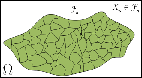
Think of some random Variable \(X_n\) and its \(\sigma\)-algebra \(\mathcal{F}_n\) (algebra of its level sets)

look at the figure above, each patch represents a “minimal” set in \(\mathcal{F}_n\). \(X_n\) gives each of those sets constant value. Namely if \(A\) is one of the patches then \(\forall \omega \in A \in \mathcal{F}_n\), \(X_n(\omega) = \alpha_{A}\).

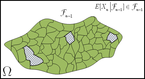
Now what is \(\mathbb{E}[X_n|\mathcal{F}_{n-1}]\)?. Note that \(\mathcal{F}_{n-1}\subseteq \mathcal{F}_{n}\) so lets think of it as -

Look how the new \(\sigma\)-algebra is more coarse, some sets that are minimal here were finer divided in \(\mathcal{F}_{n}\). \(X_n\) is not measurable on \(\mathcal{F}_{n-1}\), But \(\mathbb{E}[X_n|\mathcal{F}_{n-1}]\) is, and \(\mathbb{E}[X_n|\mathcal{F}_{n-1}]\) gives us the best guess we can make about the out come of \(X_n\). For example If on step \(n-1\), \(X_n\) happened to fall on the sets that are minimal on both \(\sigma\)-algebras then we know it cant change on step \(n\) but if it hadn’t then we will be able to narrow down possible outcomes of step \(n\) but still there will be some uncertainty, our best guess will be the ecpected value of \(X_n\) on the possible outcomes in \(n\), which is exactly the conditional expectation. Step \(n-1\) does not provide all the information but it give us the probabilities of our best guesses we will be able to do on step \(n-1\).

Technorati Tags: best guess,Conditional Expectation,Probability

Windows Live Tags: best guess,Conditional Expectation,Probability

WordPress Tags: best guess,Conditional Expectation,Probability

Probability 4 - Filtration vs Information

Forth post in the series.

How, filtration \(\{\mathcal{F}\}\) of \(\sigma\)-algebras is related to the claim “that filtration corresponds to information one has at time \(n\)”

Let me build the stage

Think of you self as been at time zero and you intend perform simple experiment where you toss coin five times in a row at times \(n=1, n=2, n=3, n=4, n=5\) and record the results. Before you toss the coin for the first time there is total uncertainty about the overall out come of the experiment, after you toss the coin for the first time you will be able to tell the result of the first toss while the rest will still remain uncertain, when you toss the coin next time you now able to tell two out comes and so on… until you completely know the result.

This process can be related to information being gaining as time passes or equivalently the uncertainty being decreasing with each toss.

So lets now turn this little bit “around” and speak of probability of you answering to the question of “what the overall result of you tossing will turnout”. This, rather weird angle of looking at the problem, will turn out to be very natural for us.

Before you toss there is probability \(1\) for you answering that every outcome is equally possible, after the first toss you will know how the coin happened to fall, so there is probability \(0.5\) of you answering that it has to be the head first and the rest is unknown and similarly with probability \(0.5\) for the tail being first while the rest is unknown. Next time you will tell with \(25\%\) chance that it is twice heads (the rest is unknown) \(25\%\) head and tail (the rest is unknown) and so on…

Ok, now, lets go back to the usual probability space of coin tossing. What  this space looks like? It is reasonable to assume that it is generated by the following sets:

\(\{\emptyset, \Omega, (00000), (00001), (00010), (00100), (01000), (10000), (00011), (00101),\dots,(11111))\}\)

Now what model we can adopt for the “space of probabilities of your answers”?

Check this out:

At time \(n=0\) we have \[\{\emptyset, \Omega, \{(00000), (00001), (00010), (00100),\\ (01000), (10000), (00011), (00101),\dots,(11111)\} \}\], pay attention to the addition of the curly brackets “\(\{\)” and “\(\}\)” we regard all the outcomes between them as single element! So actually we can write it as \(\{\emptyset, \Omega\}\) since \(\{(00000), (00001), (00010), (00100), (01000), (10000), (00011), (00101),\dots,(11111))\} \) just equals to the whole of \(\Omega\) so no need to write it twice.  Lets designate \(\sigma-algebra\) generated by this set as \(\mathcal{F}_0\).

You probably know see where its all going…

\(\mathcal{F}_1\) will be generated by \[\{\emptyset, \Omega, \{(00000), (00001), (00010), (00100), (01000), (00011), (00101),\dots,(01111))\},\\\{(10000), (10001), (10010), (10100), (11000), (10011), (10101),\dots,(11111))\} \}\] and so on.

Note: that \(\mathcal{F}_0 \subseteq \mathcal{F}_1 \subseteq  \mathcal{F}_2 \subseteq \dots \subseteq   \mathcal{F}_5 \subseteq \mathcal{F}\).

Now I will let the fog to dissipate:

The answer

Algebras (set of sets) \(\mathcal{F}_n\) encode the possible questions that can be answered at time \(n\) (indeed at time \(n=1\) we can only ask what was the outcome of the first toss so the elements in \(\mathcal{F}_1\) are build by alternating first toss) while the measure defined on this algebra gives the probability for various answers. In this regard filtration encodes also that as time will go by the number of possible answers will increase decreasing the “uncertainty”.

Probability 3 - Inequalities

Third post in the series. 

Here is the summary of various inequalities:

Jensen's inequality

It relates the value of a convex function of an integral to the integral of the convex function. if \(X\) is a random variable and \(\phi\) is a convex function, then

\[\phi(\mathbb{E}[X])\leq\mathbb{E}[\phi(X)]\].

Markov's inequality

Let \(X\) be a random variable and \(a>0\)

\[P(|X| \geq a) \leq \frac{\mathbb{E}[|X|]}{a}\]

Chebyshev’s inequality

Let \(X\) be a random variable with finite expected value \mu and finite non zero variance \sigma^2. Then for any real number \(k>0\)

\[P(|X-\mu| \geq k\sigma) \leq \frac{1}{k^2}\]

or written differently: \[P(|X-\mu| \geq k) \leq \frac{Var(X)}{k^2}\]

Chebyshev's inequality follows from Markov's inequality by considering the random variable \((X-\mathbb{E}[X])^2\)

Technorati Tags: Inequality,Probability,Jensen,Markov,Chebyshev

Windows Live Tags: Inequality,Probability,Jensen,Markov,Chebyshev

WordPress Tags: Inequality,Probability,Jensen,Markov,Chebyshev

Blogger Labels: Inequality,Probability,Jensen,Markov,Chebyshev